Introduction*
This series investigates the persistent problem of racial residential segregation in the San Francisco Bay Area by applying novel research methods and fresh analytical tools to better understand the extent and nature of the problem. The first research brief in this series described patterns of segregation in the Bay Area using a relatively new measure of segregation and illustrated these patterns using the first-ever maps of the region, counties, and major metropolitan areas with that measure. The second brief in this series examined the demographic patterns that lay behind the reality of segregation. It explored the contemporary patterns of residential settlement by race and examined changes in those patterns over time.
In this third brief, we shift the discussion to a more technical, but no less important, matter: the measurement of segregation. As we emphasized throughout this series, racial segregation is not the same thing as racial demographics. Too often, maps of racial demographics are used as a substitute for mapping segregation itself.1 In an increasingly multiracial and multiethnic society, where the presence of any particular racial or ethnic subgroup may range from small to substantial, no single demographic map can adequately represent segregation itself. Segregation is relational, dependent on the overall demography of the region examined.2 Racial diversity can mask or obscure the persistence or degree of racial segregation, especially for particular marginalized groups. As we demonstrated in Part 1, there are ways to measure and map segregation directly.
In addition to the inherent complexities of measuring segregation in an era of demographic diversity, the concept of segregation itself is multifaceted. Segregation can appear on a map like a yin-yang symbol, with large swaths of a region dominated by a particular racial group, or like a checkerboard, with racially homogeneous neighborhoods and communities clustered separately across a racially diverse region. Although substantial numbers of particular racial groups may now live in integrated neighborhoods, the average member of those groups may nonetheless remain segregated. Separate and distinct measures are needed to analyze these different realities.
Along with a mounting body of original research into the causes and effects of segregation in recent years,3 there are a growing number of measures developed to assess the degree or extent of segregation. All told, we have uncovered nearly two dozen measures used to try to gauge or quantify segregation, each with its own value and insights. By examining several measures of segregation in juxtaposition, we can offer a better-rounded portrait of the actual reality of segregation itself and a better understanding of the perspective that any particular measure illuminates—a partial glimpse of a complex whole.
Some measures of segregation show improvement while others indicate stagnation or worsening conditions. For example, the most widely used measure shows that racial segregation has declined substantially since 1970 while remaining at a high level nationwide. On the other hand, economic segregation has grown significantly in the last 50 years.4 We need an array of instruments and tools to understand all of the facets of this complex, but profoundly important, phenomenon. This brief seeks to overcome many of these challenges in measuring segregation.
This brief has two purposes. First, we seek to describe the insights offered by each measure of segregation while making the case for our preferred measure. We will survey the more popular and widely used measures of segregation, explaining their purpose and function and compare them to our preferred measure, the Divergence Index. In the process, we will explain how the Divergence Index functions in more detail and how it differs from these more popular measures. We will also highlight the advantages and drawbacks of these various measures, describing what they reveal and conceal and, where possible, the national trends.
Second, we will develop a better portrait of the dynamics of racial segregation in the Bay Area by juxtaposing these various measures. Thus, we will compare the results of the Divergence Index with several more common measures of segregation and examine how the Bay Area has evolved or changed over time.
In addition to presenting charts that illustrate these trends and findings, the main contribution of this brief is an interactive web tool that allows users to toggle between various measures of segregation and observe changes in the level of segregation with each measure over time. We also provide interpretative observations about what these results mean and signify for our understanding of the reality and dynamics of racial segregation. In the end, we hope to convey a clearer and more vivid understanding of the multifaceted reality of segregation in the Bay Area.
Defining Segregation
Broadly speaking, segregation is the separation of one or more groups of people from each other on the basis of their group identity.5 While seemingly straightforward, this concept is a minefield of nuance, subtlety, and complexity.6 Because segregation is associated with a host of complementary or corollary concepts, it is often conflated with them. As we saw in Part 1 of this series, segregation and diversity are not the same thing. Diverse cities, such as Oakland and Berkeley, are also highly segregated in spite of their diversity. A place can be diverse and segregated, or neither, or one but not the other.7
Similarly, “segregation” has certain connotations that can lead to confusion when using the term in a more precise way. Typically, “segregated neighborhoods” or “segregated schools” refer to predominantly Black or Latino schools. But, as noted in Parts 1 and 2, predominantly white schools and neighborhoods can be just as segregated, if not more so. In fact, it is difficult to imagine how Black schools in the Jim Crow south could be described as segregated, but the all-white schools not similarly characterized.8 They were both segregated using the same means, although they are segregation of a different sort.9
Another source of confusion is that racial segregation is not a totalizing, all-encompassing experience. A place can be both segregated and integrated at the same time. The explanation for this paradox is that segregation can occur in certain domains, such as schools or neighborhoods, but not in others, such as job sites, public transit, or other public facilities. It is possible for public spaces to be integrated while residential spaces are segregated, and vice versa. That is why this series has restricted its focus primarily to residential segregation, which is “the degree to which two or more groups live separately from one another, in different parts of the urban environment.”10
One of the more recent contestations over the term “segregation” concerns its legal significance and whether it refers to patterns of racial separation that result from private decisions, so called de facto segregation, or only to government created or caused segregation, known as de jure segregation. In a 2007 Supreme Court decision concerning two “voluntary” integration plans concerning K–12 student assignment in school districts in Seattle, Washington, and Louisville, Kentucky, the justices of the Supreme Court debated this question.11
In concurring with the majority of the Court, Justice Clarence Thomas wrote a separate opinion in which he declared that “contrary to the dissent’s rhetoric, neither of these school districts is threatened with resegregation […]. Racial imbalance is not segregation, and the mere incantation of terms like resegregation and remediation cannot make up the difference.”12 According to Justice Thomas, “segregation is the deliberate operation of a school system to ‘carry out a governmental policy to separate pupils in schools solely on the basis of race’ (Swann v. Charlotte-Mecklenburg Bd. of Ed., 402 US 1, 6 [1971]).” On the other hand, he defined “racial imbalance [as] the failure of a school district’s individual schools to match or approximate the demographic makeup of the student population at large.”13
This was more than a mere semantic debate. Under prevailing (but not necessarily correct) interpretations of the Constitution, government responsibility to remedy segregation extends only to that segregation it has caused or contributed toward producing. The sharp distinction between “racial segregation” and “racial imbalance” drawn by Justice Thomas functions to shield state or local government from responsibility for remediating it while also making it more difficult for school districts (and other government decision-makers) to address de facto segregation with race-conscious remedial attendance plans or other diversity-enhancing measures.
In the concurring opinion providing the crucial fifth vote, however, Justice Anthony Kennedy rejected the sharp distinction drawn by his more conservative colleagues in the plurality. He recognized that federal, state, and local government policy, past and present, is inextricably intertwined with private, voluntary housing decisions, in both the shaping of individual preferences and structuring of the private market to produce patterns of residential racial segregation that persist today. As he explained, “[t]he distinction between government and private action […] can be amorphous both as a historical matter and as a matter of present-day finding of fact. Laws arise from a culture and vice versa. Neither can assign to the other all responsibility for persisting injustices.”14 We agree with this view.
While it is possible for patterns of residential racial segregation to be entirely voluntary—a product of individual preferences completely untainted by government policy—this is unlikely. Even if current patterns of segregation are not compulsory, in the sense of being mandated by legislative fiat, as was the case under Jim Crow, it is still the case that segregation is not entirely a choice in the sense that the word “voluntary” implies. Not only has past governmental policies structured housing preferences by promoting segregation, but contemporary housing policies tend to reinforce those patterns and, thus, indirectly cause segregation as a forced response to the lack of other options available. Therefore, we define segregation as encompassing both de facto and de jure forms of segregation, and we reject a sharp distinction between them. Past and present-day government policies contribute to racial segregation and cause racial isolation.
One additional subtlety bears explicating regarding the purpose or function of segregation and how it is accomplished. Although “segregation” is defined as the separation of groups of people from each other in various domains of life, the purpose of segregation is not simply to keep people apart. Rather, the purpose of segregation is to control access to, or the distribution of, communal resources, public and private, what the great sociologist Charles Tilly called “opportunity hoarding.”15 Thus, segregation—whether on the basis of race, religion, or gender—is not simply about separating people for its own sake; it is about controlling access to opportunity and other life-enhancing resources and capacities.
In that regard, the notion that segregation harms children of color in primary and secondary education does not reflect an assumption that such children are incapable of learning if racially segregated. Rather, it reflects the presumption that resources, tangible and intangible, will be inequitably distributed or afforded in segregated educational settings. Thus, the US Supreme Court recognized, in the case of gender-segregated educational military institutions, that even if tangible resources were equalized, intangible resources, such as prestige, alumni networks, and social capital, might not be.16
As uncomfortable as it may be, and as much as we might try to make it otherwise, it is unlikely that racial inequality will ever be significantly reduced, let alone eliminated, in a racially segregated society.
Popular Measures of Segregation
Segregation is a surprisingly difficult concept to measure and map. In addition to the subtleties and complexities just noted, another nuance to segregation is that the spatial patterning can be described in several different ways. Over the years, a variety of measures have emerged, each seeking to address one or more problems with previous measures. In their landmark book American Apartheid, Douglas Massey and Nancy Denton describe segregation in five different ways: (un)evenness, exposure, concentration, centralization, and clustering.17 Some of these ways of describing segregation have different measures.
The most commonly used and widely cited measure of segregation is “evenness,” or ”spread,” and is known as the Dissimilarity Index. This index indicates the number of people of either racial group that would have to move to integrate the community. The Dissimilarity Index is scored from 0 to 100 (or 0 to 1), with 0 indicating perfect integration and 100 (or 1) indicating complete segregation. At the national level, the United States scores a 59 according to the 2010 Black-white Dissimilarity Index, meaning that 59 percent of whites or Blacks would have to move to achieve perfect integration. The Bay Area fares somewhat better on this measure, depending on the metropolitan statistical region (MSA) being examined.
As of 2010, the San Francisco-Oakland-Fremont Black-white dissimilarity score was also 59, the same as the national average.18 However, the San Jose-Sunnyvale-Santa Clara Black-white dissimilarity score was only 38.6.19 For the San Francisco-Oakland-Fremont MSA, the white-Latino dissimilarity score was 49.6, and the white-Asian score was 44.3, showing a high level of racial segregation. However, the San Jose-Sunnyvale-Santa Clara white-Latino score was higher than that for Blacks, with 47.6, as was the white-Asian score of 43. Both Asians and Latinos in the San Jose MSA are more segregated from whites than Blacks. So the Black-white dissimilarity score is not indicative of the degree of segregation from whites for other groups. Nor could you infer the degree of segregation experienced by Blacks from the Asian or Latino dissimilarity scores vis-à-vis whites.
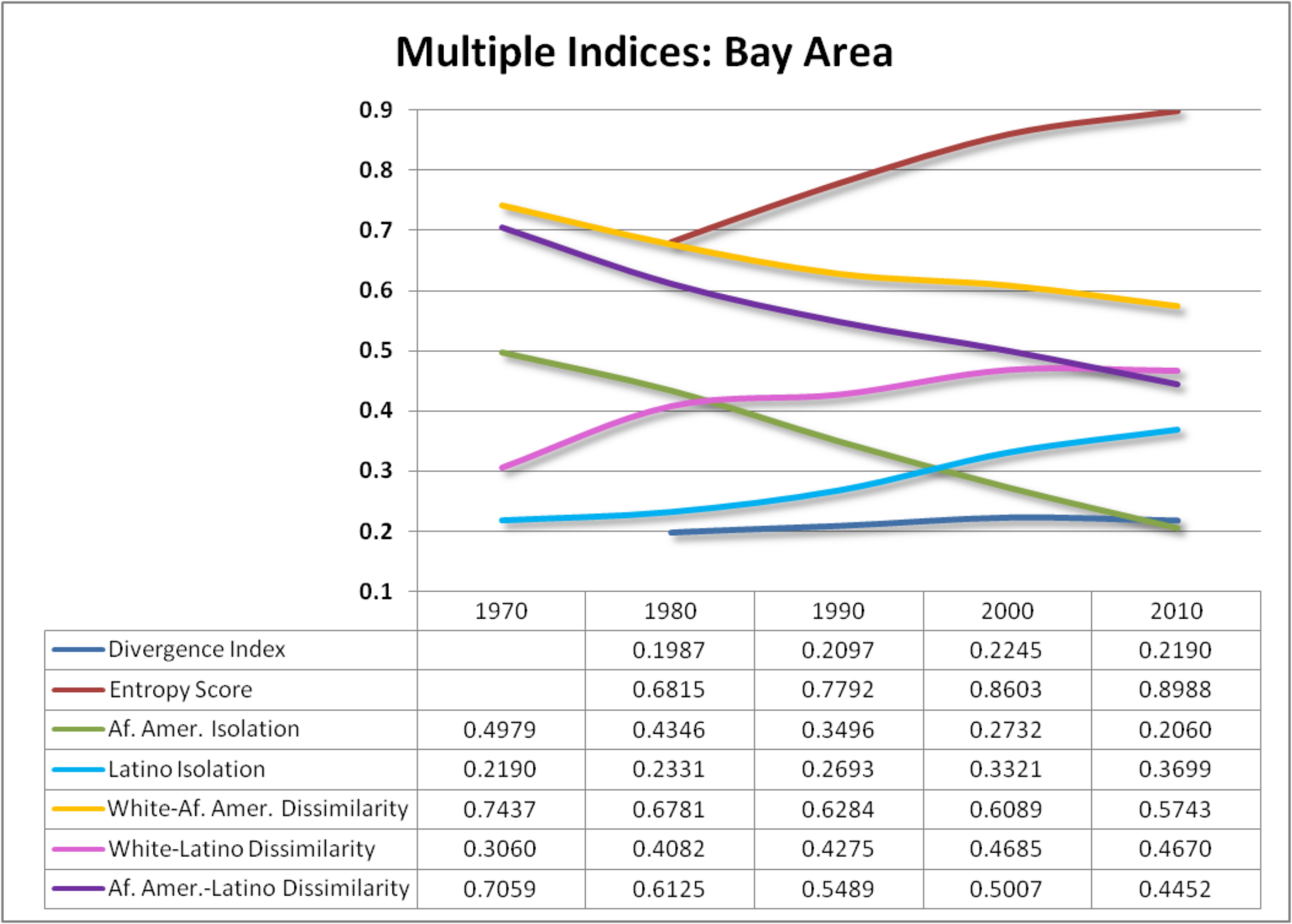
As has been true nationally, Bay Area Black-white dissimilarity scores have fallen in recent decades (see the following table). Black-white dissimilarity scores were very high as of 1970, at 0.74, suggesting that nearly three-quarters of either Blacks or whites would have to move to a different neighborhood to achieve integration. From 1970 to 2010, the Black-white dissimilarity score fell by 0.17.20 A greater portion of that decline occurred from 1970 to 1980, where it fell by 0.07, which would put it nearly in line with metropolitan areas nationally that had moderate declines in segregation, including Atlanta, Dallas, Los Angeles, and Nashville, but not quite as precipitous as those metropolitan areas with large declines in the same period, such as Seattle, San Diego, Oklahoma City, and Minneapolis.21 Moreover, the rate of decline has slowed over time, such that Black-white segregation, according to the Dissimilarity Index, appears to have stabilized.
More critically, however, white-Latino segregation appears to have intensified and is on an upward trajectory, growing from a relatively moderate level of 0.41 in 1980 to 0.467 in 2010, an increase of nearly 0.06, virtually the same amount that segregation fell between whites and Blacks from 1970 to 1980. This suggests that Latinos are increasingly concentrated into racially isolated neighborhoods, which may partly be a by-product of large increases in overall Latino population.22
This begins to illustrate one of the limitations of the Dissimilarity Index. Areas with more overall racial diversity tend to show lower overall Black-white dissimilarity scores—not necessarily because Blacks and whites are more integrated, but because there are fewer all-white or all-Black neighborhoods. Indeed, the greatest reduction in the dissimilarity scores in the chart below is between Blacks and Latinos, whose levels of intergroup segregation fell from 0.71 in 1970, almost as high as white and Black segregation, to 0.45 in 2010—a precipitous decline.
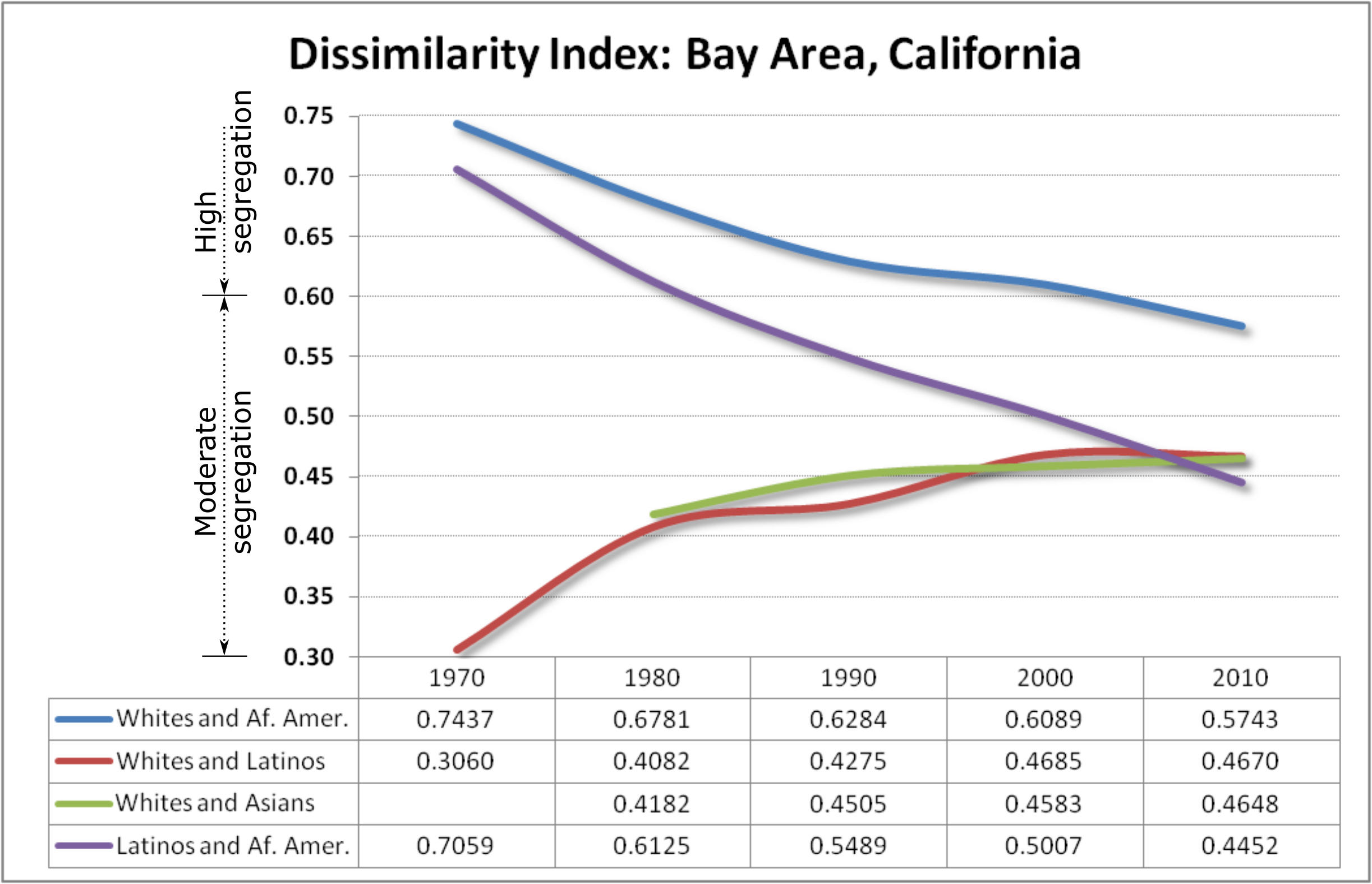
In summary, Black-white dissimilarity has declined significantly from 1970 but remains at a moderately high level, and at a higher overall level than that of any other two groups. And although Black-white and Black-Latino dissimilarity has declined over time, those declines have been matched by increases in white-Latino and white-Asian dissimilarity. In short, Black-white segregation has improved but is still quite bad, while white-Latino and white-Asian segregation is moderate but getting worse.
Another measure of segregation is known as the Isolation Indices, which includes both the Isolation Index as well as the Exposure Index. These indices measure the flip sides of each other and seek to calculate the degree of “exposure” or isolation experienced by the average member of a particular racial group. Rather than looking at overall patterns, the Isolation Indices focus on the typical case. For example, an Isolation Index score of 50 would suggest that the average African American resides in a neighborhood that is 50 percent Black, and a Black-white Exposure Index score of 30 suggests that the average African American lives in a neighborhood that is 30 percent white.
In several respects, the Isolation Indices are a superior measure of segregation to the Dissimilarity Index. While a significant number of African Americans have integrated previously all-white neighborhoods—causing much of the decline in the Black-white dissimilarity score— many African Americans reside in segregated neighborhoods. By focusing on the average member of a race, the Isolation Indices give us a different, perhaps more relevant, sense of how segregated a particular racial group remains.
Nationally, African Americans in 2010 have an Isolation Index score of 35, which means that the average African American resides in a neighborhood that is 35 percent Black. For African Americans in the San Francisco-Oakland-Fremont MSA, that number was 23, not quite as concentrated, but still quite high relative to their proportion of the population. The average Black resident resided in a neighborhood that was 23 percent Black, 28 percent white, 27 percent Latino, and 22 percent Asian. This would seem quite diverse. The problem is that the average white resident in that MSA resides in a neighborhood that is 6 percent Black, 16 percent Latino, 22 percent Asian, and 56 percent white. Thus, the whites and Blacks in the Bay Area appear to reside in demographically different worlds.
This is also true of Latinos and Asians. As of 2010, Latinos in the San Francisco-Oakland-Fremont MSA resided in a neighborhood that was 36 percent Latino, 30 percent white, 11 percent Black, and 22 percent Asian. And Asians in that same time period and MSA resided in a neighborhood that was 39 percent Asian, 8 percent Black, 18 percent Latino, and 35 percent white.
The Isolation Indices show, however, that Latinos and Blacks are less segregated from each other today than a generational ago, as was also suggested by the Dissimilarity Index. Latinos have moved into previously all or majority Black neighborhoods in large numbers in recent decades.23
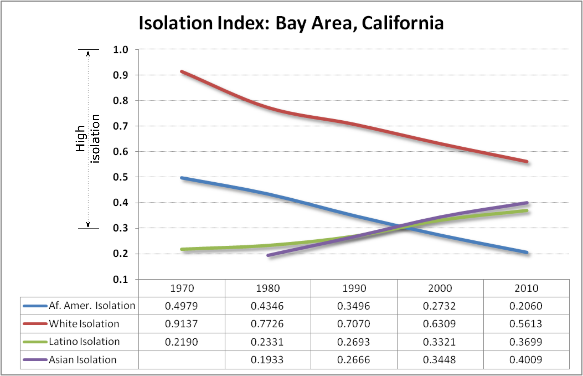
The following chart shows how isolation scores for each of the four major racial-ethnic groups have changed over time in the Bay Area. Whites and Blacks are substantially less isolated than they were a generation ago because there are far fewer all-Black and all-white neighborhoods, but they still remain fairly isolated. In fact, although whites are just 40 percent of the population of the Bay Area, they remain the most racially isolated group, as noted in Part 1. Whites continue to have very low exposure to Blacks and relatively low exposure to Latinos in the Bay Area.
It bears further noting, however, that Latino and Asian isolation—and therefore racial segregation—is gradually increasing, with a sharp increase in Asian and Latino isolation from 1970 to 2010. This cannot be simply a result of immigrants moving into ethnic communities, but rather a more structural force, since the rate of increase remains the same through various waves of immigration illustrated in Part 2.
Both the Dissimilarity and Isolation Indices reflect persistently moderate to high levels of racial segregation, despite some improvements and some deterioration toward integration and demographic milieus that are starkly different. Although Dissimilarity and Isolation Indices appear to be trending in the same direction, they reflect different kinds of information. The former measures how separated individual groups are from each other, while the latter examines the demographic composition of the neighborhood average, or typical member, of each racial group.
While revealing different facets of the reality of segregation, each index masks others. The Dissimilarity Index masks the persistence of segregation of the typical member of each racial group and the demographically divergent realities of their respective environments, while the Isolation Indices mask variation from the norm because they focus on the average neighborhood for each racial group. Most critically, however, both the Dissimilarity and Exposure Indices only measure groups from a relative position against each other. For that reason, we must turn to measures of multigroup segregation.
Measuring Multiracial Segregation
The indices previously described provide important insight into the phenomena of segregation, but primarily for two racial groups at a time, and for a larger geography, such as a municipality, county, MSA, or region. The desire to measure segregation for smaller geographies, such as census tracts, as well as to examine segregation for multiple groups simultaneously, led social scientists and demographers to develop additional metrics. These metrics include the Entropy Score and the Divergence Index—the two that we will focus on.
The Entropy Score measures the diversity of an area, be it a metropolitan area or a census tract, by assessing the representation of each racial group within that area.24 We can assess diversity (Entropy Score) of any geography as long as we have data for each racial group, and these groups are mutually exclusive.25 For example, to calculate the entropy score for a county or a region, we need to have data on proportions of each of those mutually exclusive groups within the geography. To illustrate how this works, here are the population numbers of some of the racial groups in Alameda County and a census tract within that county.26
|
Tract |
Tract proportions |
Alameda County |
County proportions |
|
|---|---|---|---|---|
|
White |
295 |
0.093 |
679,465 |
0.616 |
|
Black |
2,422 |
0.76 |
200,832 |
0.182 |
|
Latinos |
380 |
0.119 |
129,566 |
0.117 |
|
Asians |
88 |
0.028 |
93,730 |
0.085 |
|
Total |
3,185 |
|
1,103,517 |
|
Tract entropy (scaled) score (Ei) = 0.56
County entropy (scaled) score (E) = .7727
The following chart shows the entropy scores disaggregated by county, but also for the entire Bay Area, over time.
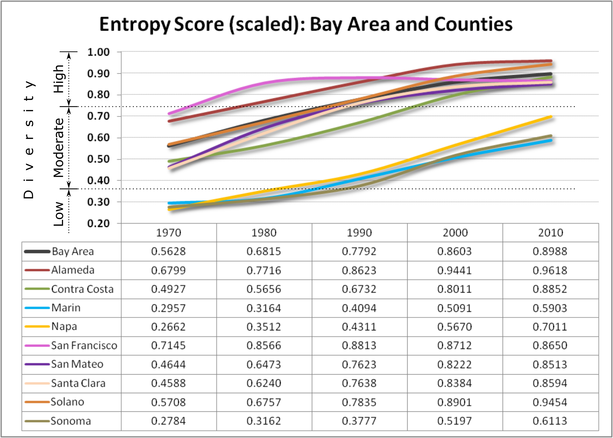
However, critics point out a few issues with the Entropy Score. First, the entropy score seems to capture diversity more than segregation itself.28 The chart above shows that entropy scores change with levels of diversity in each county. But as we warned earlier, a place can be diverse and still highly segregated.
Secondly, the Entropy Score assigns the highest score to perfectly equal racial group proportions, without giving context to the larger geography's demographics. Given the varying levels of racial representation across the Bay Area, this can be quite misleading.
This leads us to another index, more recently developed by Elizabeth Roberto and which we featured in Part 1 of this series, known as the Divergence Index.29 We believe it is also more intuitive to understand. Where the Entropy Score measures relative diversity, the Divergence Index measure segregation at any geographic level and, thus, better matches the common sense definition of segregation.30 The Divergence Index measures the degree of “divergence” in demographics from a particular geography to another larger geography, such as a census tract to a county.31
As a proponent of this index explains, “What distinguishes the concept of diversity from segregation and inequality is its indifference to the specific groups that are over- or underrepresented in a population. Diversity measures are only concerned with the variety or relative quantity of groups, whereas inequality and segregation measures are concerned with which groups (or which parts of a distribution) are over- and underrepresented.”32
Let us illustrate this using our example from the previous section. Below is a table with race data in 1980 for a tract within Alameda County.
|
Tract |
Tract proportions |
San Francisco-Oakland-Berkeley CBSA |
CBSA proportions |
|
|---|---|---|---|---|
|
White |
295 |
0.093 |
2,164,616 |
0.667 |
|
Black |
2,422 |
0.760 |
384,700 |
0.119 |
|
Latino |
380 |
0.119 |
351,900 |
0.108 |
|
Asian |
88 |
0.028 |
344,965 |
0.106 |
|
Total |
3,185 |
|
3,246,181 |
|
Divergence Index for tract33 = 1.21
This shows that this census tract is highly segregated, as the relative tract and core-based statistical area (CBSA) demographics suggest.34
An important characteristic of the Divergence Index is that it directly compares one racial group’s proportions to its CBSA proportions. This is an advantage over the acontextual approach of Entropy Score.
The following chart illustrates the divergence scores for each county and for the entire Bay Area, from 1980 to 2010.
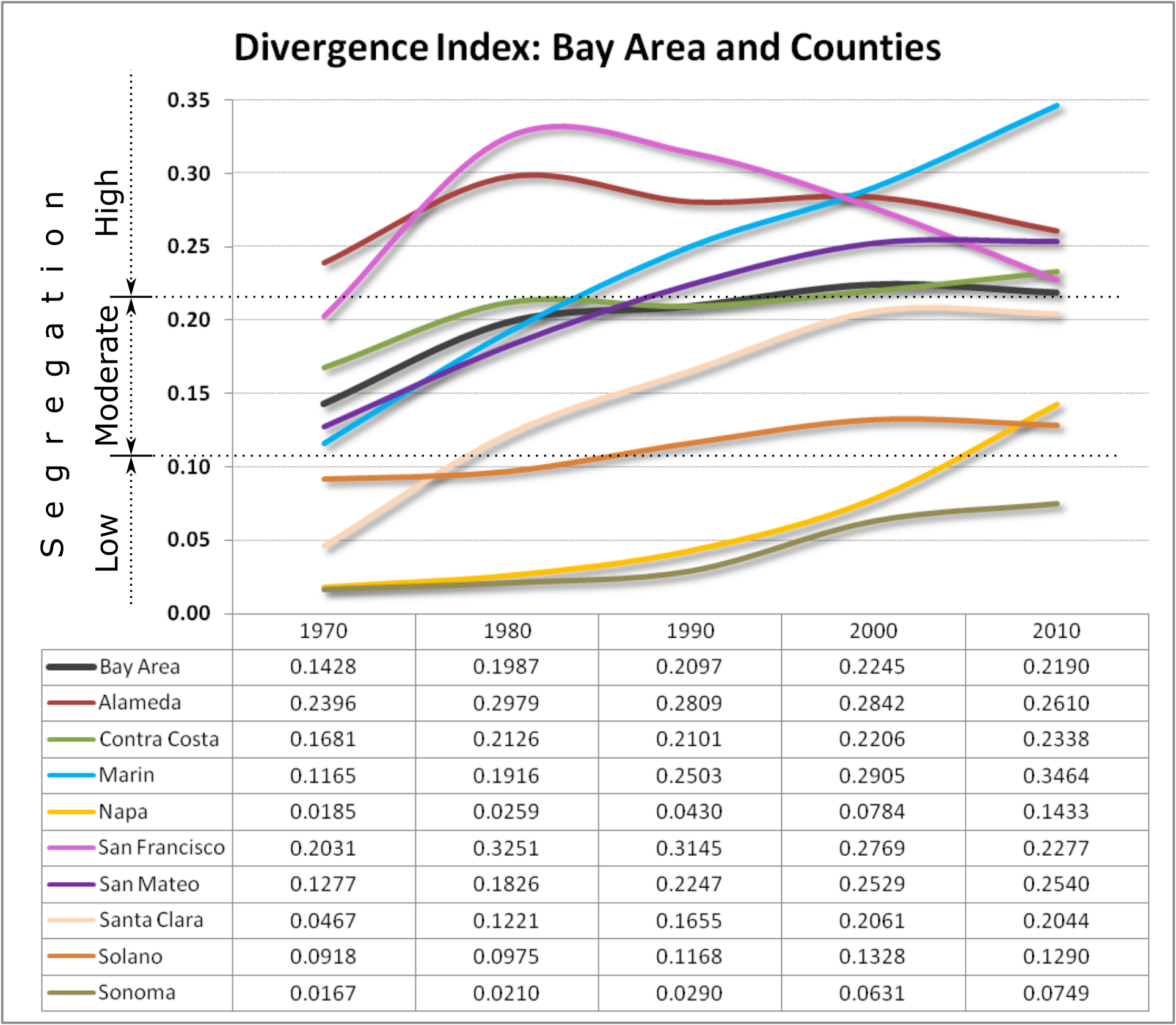
Using the thresholds created for Part 1 of this series,35 the entire Bay Area is borderline highly segregated as of 2010, but the level of segregation has risen since 1980, rather than fallen, as other measures suggest. This aggregate calculation, however, conceals considerable variation at the county level.
Some counties, such as San Francisco, have shown substantial reduction in segregation since 1980 but are still in the “High segregation” zone. Other counties, such as San Mateo, have gone from moderately segregated to nearly high levels of segregation during the same period.
Alameda and San Francisco can be classified as being highly segregated under this index since 1980, though both counties display substantial decline in segregation. Perhaps most concerning, all but two of the nine counties have had increases in segregation under this measure since 1980, though Contra Costa and Solano display moderate level of increase within the same time period. And, in fact, in many cases, the increases in levels of segregation have been relatively large (such as in Sonoma, Napa, Marin, and Santa Clara), even if the final value is at a relatively low or moderate level. Thus, Marin has had a twofold increase in the level of segregation, even if the initial level was fairly moderate. The level of segregation in Sonoma has nearly quadrupled. These findings complicate the overly simplistic and optimistic portrait of segregation suggested by the Dissimilarity and Isolation Indices.
To confirm our conclusions that the level of segregation in the Bay Area observed with the Divergence Index is increasing over time, we used American Community Survey data collected in 2017 (the latest year available), and found this to be true. In fact, we found an overall nine-county Bay Area Divergence score of .234, the highest ever observed for the region. We also found that eight of the nine counties had higher Divergence scores in 2017 using ACS data than in 2010 using decennial census data. We look forward to the 2020 census results where we can get more definitive and accurate estimates. But this shows that divergence scores as of 2017 are consistently higher than 1970.
Comparing and Contrasting Segregation Indices in the Bay Area
Given the multiplicity of indices that exist for measuring segregation, and the sometimes significant and subtle differences between them, it is useful to juxtapose the results to create a more holistic portrait of segregation in the Bay Area. While the absolute scores matter, the trending direction matters just as much. We need to know both the direction of the trend—progress or regress—and we need to know how much or how fast conditions are improving or regressing.
If we looked only at dissimilarity or isolation scores, we might have some cause for optimism. After all, as we saw above, there have been significant declines in Black-white dissimilarity segregation and Black and white isolation since 1970. Although the rate of decline has slowed substantially, the direction is still positive, toward integration. Still, there are reasons to be concerned. As we said, both Asian and Latino isolation are increasing, and white-Latino dissimilarity is also sharply increasing.
Even the entropy scores, which look more at diversity than segregation—and which, sadly, are far more frequently used—overstate the degree of progress we’ve made. In fact, the Bay Area perfectly illustrates the limitations of the Entropy Score. Since it is such a diverse place, it is showing vast improvements more attributable to increasing multiracial diversity than to integration.
It is only when we look at divergence scores that a full portrait of the changes in levels of segregation becomes manifest, as we saw earlier. Divergence scores suggest that segregation has increased, on the whole, since 1980.36 But to more vividly illustrate the contrast, we present the following charts that juxtapose the various measures of segregation we have reviewed in this brief. We begin by doing this for Alameda County.
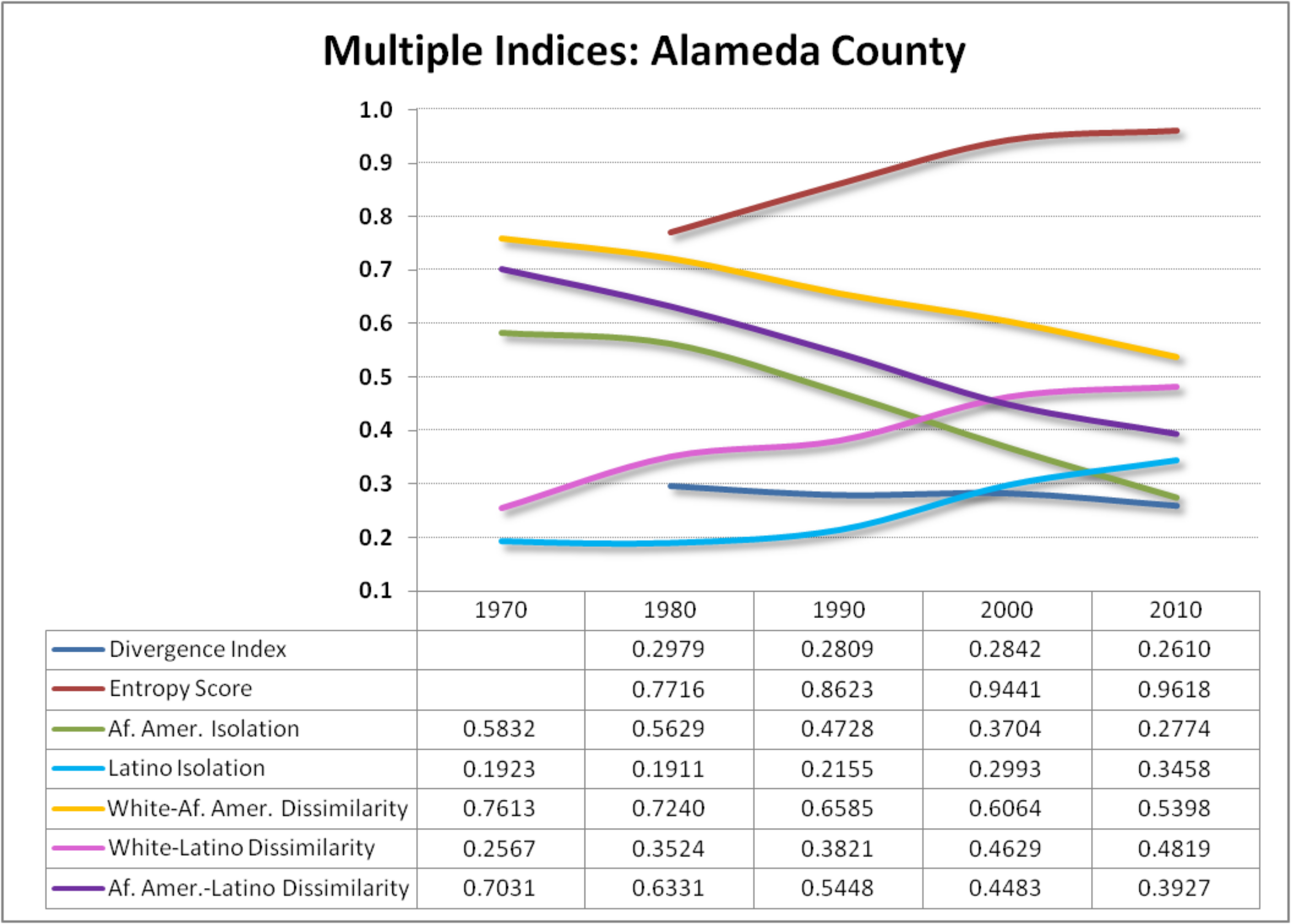
As this chart shows, racial segregation has changed very little since 1970, and remains almost exactly at the same level. It worsened a bit and improved a bit in intervening decades, depending on the decade, but the levels are uniformly similar. Alameda County’s divergence score has remained remarkably stable over the four decades examined here, even as Black-white dissimilarity and Black isolation scores have declined steadily. Entropy scores for Alameda County show a much sharper decline.
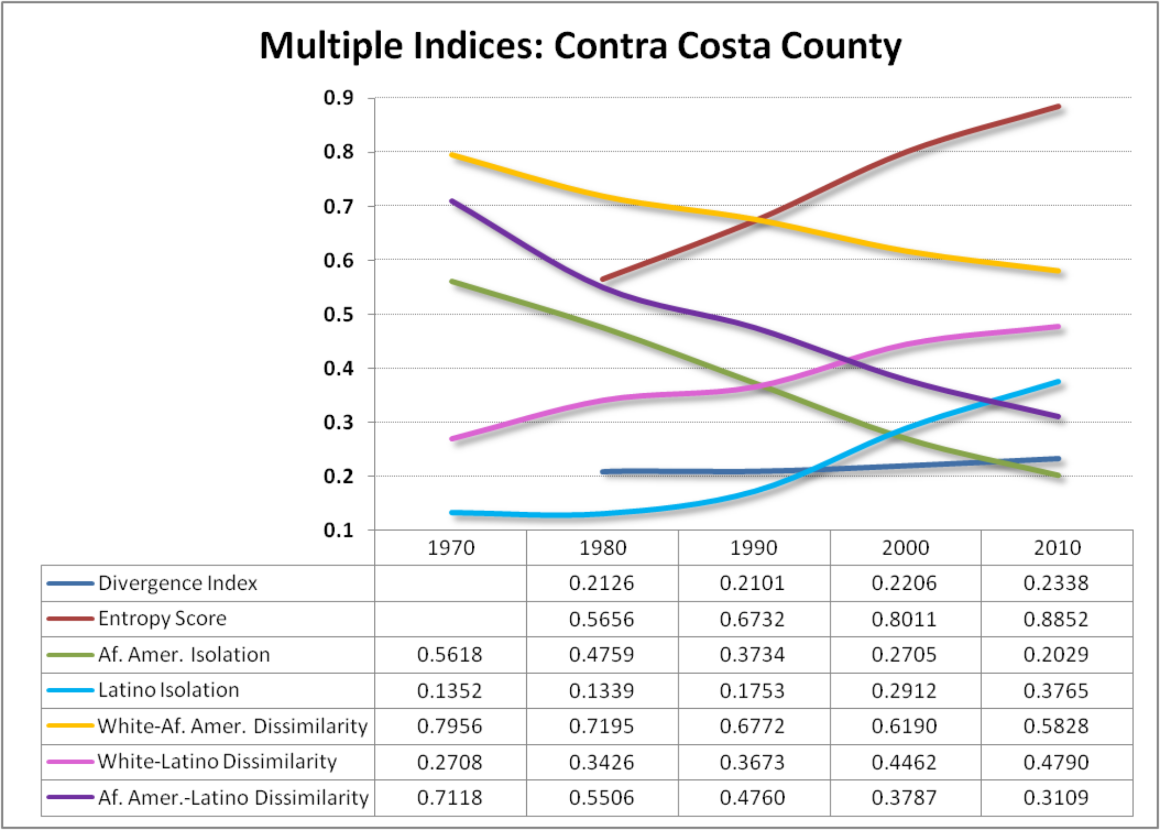
Next, consider Contra Costa County in the following chart, which shows a story similar to that of Alameda: slightly increasing segregation using the Divergence Index, settling at a moderate to high level of segregation, while Black-white dissimilarity and Black isolation steadily decline, but dissimilarity still remains at a high level. In fact, despite the sharp increases in white-Latino dissimilarity scores, Black-white dissimilarity is still the highest, meaning that Black-white segregation is still the most intense.
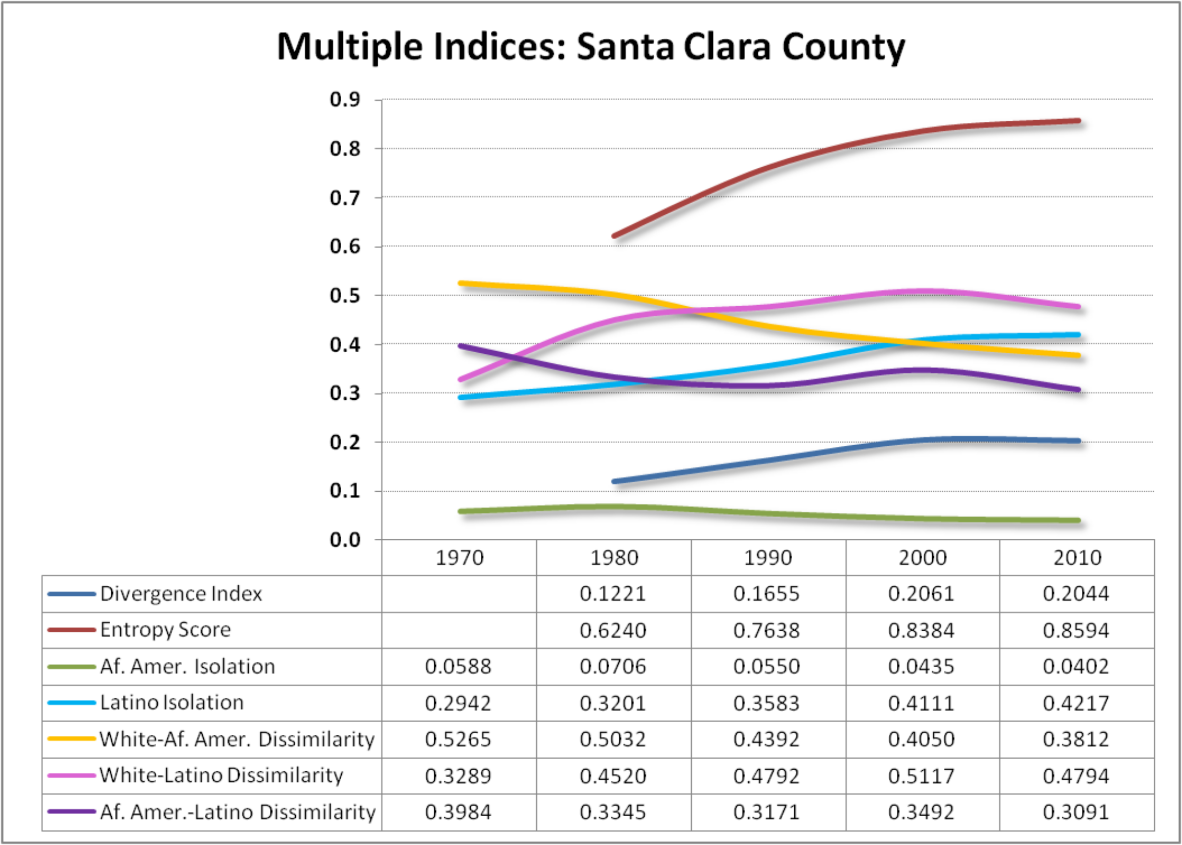
Santa Clara County, which houses the region’s largest city, has very different demographics but also tells a similar story. The main difference is that segregation has stabilized since 2000 while having risen since 1980. This county falls within the “moderate” category but has higher levels of segregation within the category.
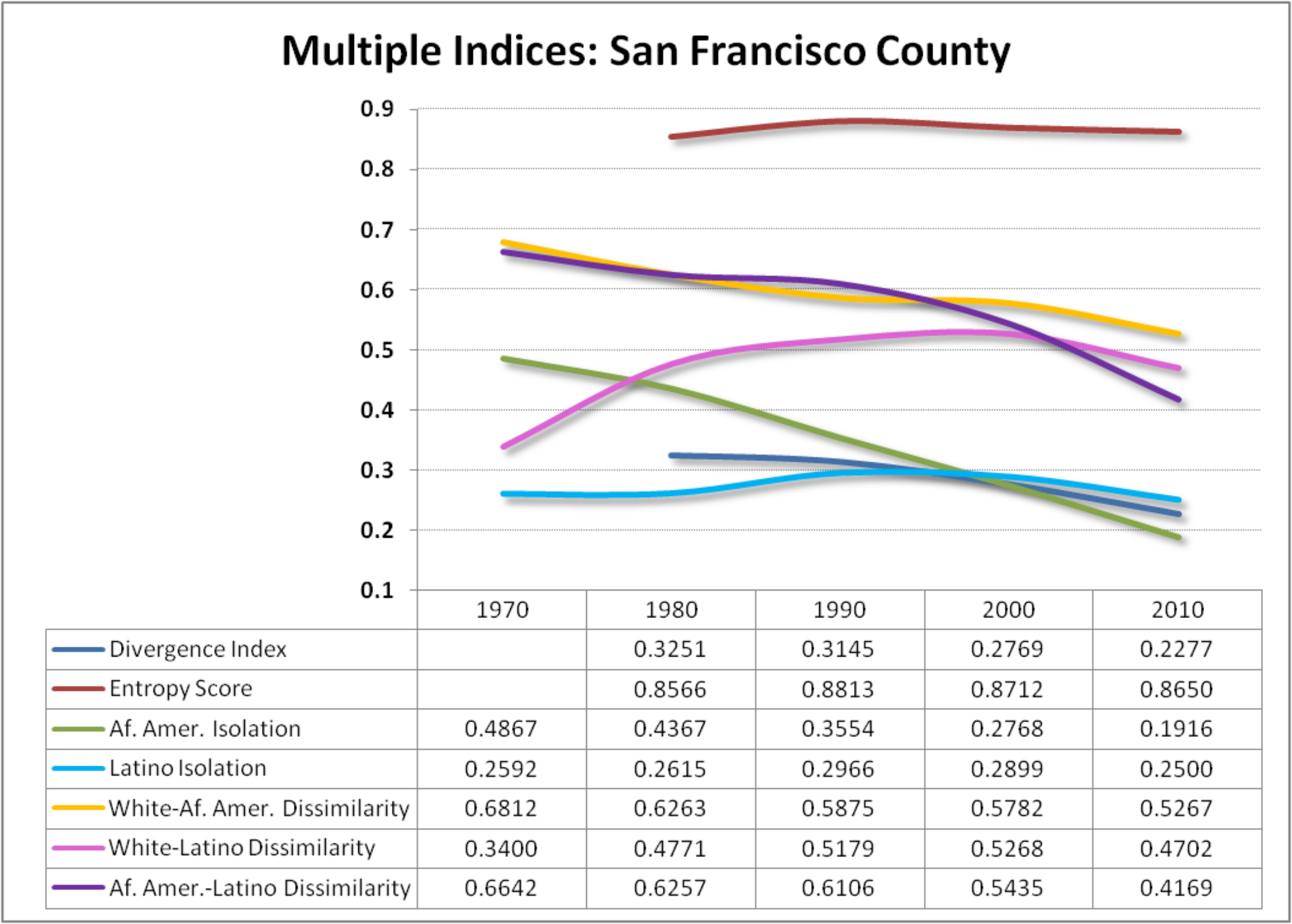
San Francisco, appears to be the county that has experienced more significant integration over the same period. This raises a provocative, but complex, set of questions about the relationship between gentrification and segregation, which we lack space to address here.
And finally, the story suggested by the county-level charts is reflected in the chart for the entire Bay Area.
Divergence scores show a region that is moderately segregated, but increasingly segregated, even as other measures show a moderately to highly segregated region, but decreasingly so.
Our analysis permits us to examine change at the neighborhood (tract) level over time, although this is easiest to observe on the interactive web map we have created to illustrate such patterns. The application allows users to toggle between different segregation indices to examine the level of segregation indicated or suggested by each index for each tract within the Bay Area. The map also lets users move a slider from one decennial census to another to see how levels of segregation have changed over time with each index.
We identified the tracts with highest increases and decreases in segregation using the Divergence Index from 1980 to 2010. The following graphic shows the neighborhoods in the inner-core of the Bay Area that experienced these changes.
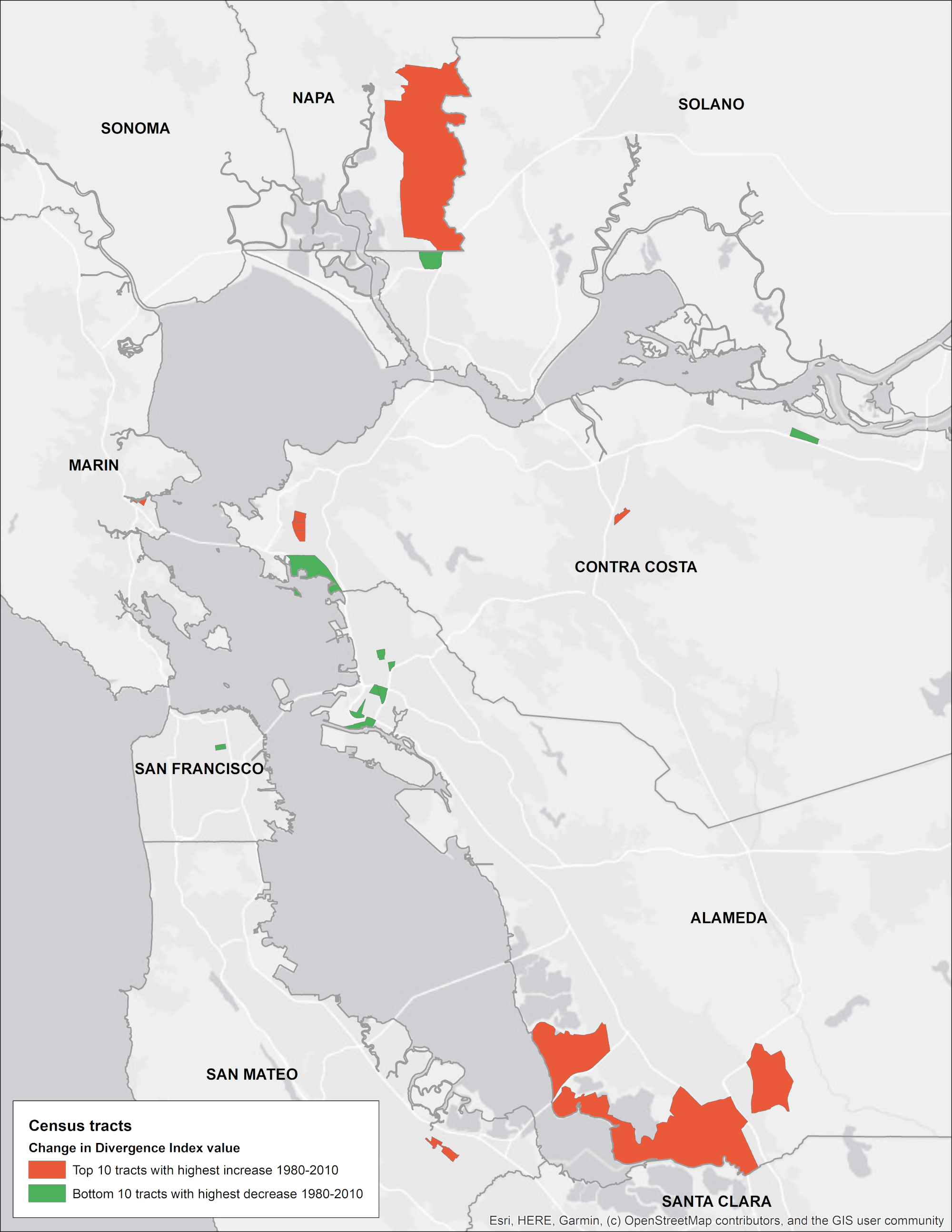
The tracts with highest increases are from five different counties: four from Contra Costa, two each from Alameda, and one each from Marin and Napa.
Seven out of 10 tracts with the largest increases show an increase in Latino population ranging from 45 to 83 percentage points. The remaining three show an increase in Asian population ranging from 40 to 74 percentage points. Six out of these 10 are the tracts that were identified as highly segregated in 2010 in our Part 1 report/analysis, where four were highly segregated for Latinos and two were segregated for Asians. In other words, there are communities with large increases in racial sub-groups.
Similarly, 10 tracts with the most significant decreases in Divergence Index values are from four counties: six from Alameda, two from Contra Costa, and one each from San Francisco and Solano. Nine of these 10 tracts show a decrease in African American population ranging from 38 to 58 percentage points. One tract in Alameda shows a decrease in Latino population by 67 percentage points.
This is consistent with the demographic shifts highlighted in our Part 2 analysis. White and African American population has declined consistently in the Bay area whereas Latino and Asian population has increased consistently since 1980. The tracts that decreased the most moved from being heavily Black to very diverse, and tracts that increased went from being heavily white to heavily Latino or Asian.
Conclusion
This brief is an answer to the challenge of measuring segregation. It is part of a series that clearly and carefully describes the pattern of racial residential segregation in the San Francisco Bay Area and illuminates the contemporary demographic patterns across spaces within the region. This brief delved into the thorny and challenging question of how to measure and represent racial segregation. We examined a few of the most popular measures of segregation, as well as some more obscure ones, but each measure provided insight into at least one facet of a complex phenomenon.
Our main findings are that the San Francisco Bay Area remains segregated more than 50 years after the passage of the federal Fair Housing Act. In fact, most counties in the region are more segregated today than they were in 1980, despite reduction in segregation between particular racial groups.
Disaggregating the data, we see that even as Black-white and Black-Latino dissimilarity scores have fallen, Asian-white and Latino-white dissimilarity scores have risen, quite significantly in some cases. Nonetheless, Black-white segregation remains the highest, even if the trends are worse in other cases. This is one of our most important findings.
The Isolation Index shows that despite some degree of integration by members of racial groups (there are far fewer racially homogeneous neighborhoods), the typical member of a racial group still resides in a demographically isolated context.
Contrary to the usual story told by falling dissimilarity scores, the Divergence Index paints a portrait of a region that is marked by persistent—and generally rising—levels of segregation. The Divergence Index shows that seven of the nine counties in the Bay Area have higher levels of segregation as of 2010 than they did in 1980. Some counties, such as Napa, Sonoma, and Marin, are dramatically more segregated than they were in 1980.
We hope that this research conveys the importance of multi-index approaches to examining the enduring problem of segregation. We have provided what may be the most advanced interactive segregation web map ever created to illustrate the changes in levels of segregation among each of these indices over time.
Our next brief will examine the harms of segregation. We will summarize some of the most notable findings in the social science literature on the harmful effects of segregation, and then we will present our original research findings on the relationship between higher levels of segregation and a variety of life outcomes.
- *The authors would like to acknowledge Arthur Gailes for creating and coding the interactive webpage that is a part of this report and for his research. The authors would also like to acknowledge Richard Rothstein, Andrew Beveridge, Richard Wright, John Logan and Elizabeth Roberto for their feedback.
- 1See, e.g., Tony Roshan Samara, “Race, Inequality, and the Resegregation of the Bay Area,” p. 10, Map 5. Urban Habitat, Oakland, CA, November 2016, http://urbanhabitat.org/sites/default/files/UH%20Policy%20Brief2016.pdf. See also Philip Verma, Dan Rinzler, Eli Kaplan, and Miriam Zuk, “Rising Housing Costs and Re-Segregation in the San Francisco Bay Area,” p. 6, Map 1. Urban Displacement Project, Berkeley, CA, https://www.urbandisplacement.org/sites/default/files/images/bay_area_re-segregation_rising_housing_costs_report_2019.pdf
- 2For example, in Northern Ireland, the segregation mainly occurs on a sectarian religious basis rather than a racial or ethnic basis. See Social-spatial Segregation: Concepts, Processes and Outcomes (edited by Lloyd, Christopher D., Shuttleworth, Ian G., David W. Wong), Chapter 9 “Perspectives on social segregation and migration: spatial scale, mixing and place.” Policy Press, 2015. In the United States, segregation depends on the presence of particular racial groups. In racially homogeneous areas, racial segregation may not exist.
- 3See e.g. Rucker C. Johnson, “Long-run Impacts of School Desegregation & School Quality on Adult Attainments.” NBER working paper #16664. Revised June 2015, available at https://www.nber.org/papers/w16664 See also, Jessica Trounstine, Segregation by Design: Local Politics and Inequality in American Cities. Cambridge: Cambridge University Press, 2018. doi:10.1017/9781108555722.
- 4Reardon, S.F., & Bischoff K. (2016). The Continuing Increase in Income Segregation, 2007‐2012. Retrieved from Stanford Center for Education Policy Analysis: http://cepa.stanford.edu/content/continuing-increase-income-segregation-2007-2012.
- 5See the definition of “segregation” in the Oxford English Dictionary online, accessed at https://en.oxforddictionaries.com/definition/segregation.
- 6See the “Measurement of Segregation” by the US Bureau of the Census in Racial and Ethnic Residential Segregation in the United States: 1980–2000 by Weinberg, Iceland, and Steinmetz, accessed at https://www.census.gov/hhes/www/housing/resseg/pdf/massey.pdf. See also Social-Spatial Segregation, p. 414. There has been an ongoing and unresolved debate about whether the five dimensions described by Massey and Denton (“evenness, exposure, clustering, concentration, and centralization”) are truly distinct, related, or corollaries. We do not seek to resolve that debate here, but rather suggest that each measure suggests a facet of segregation while proposing that the Divergence Index best matches the commonsense understanding of the concept.
- 7This is one of the problems we have with the brilliant MixedMetros methodology created by Richard Wright, Mark Ellis, Steven Holloway, and Gemma Catney. 2018. By relying on entropy, and supplementing it with a recognition of particular racial concentrations and clustering, the maps ultimately do not show segregation directly. See http://mixedmetro.com/.
- 8See tweet about segregation by Trevon D. Logan, accessed at https://twitter.com/TrevonDLogan/status/1099032389106495490.
- 9To try to overcome this distinction, the MixedMetro authors distinguish between “low diversity” white tracts and “low diversity” Black or Latino tracts. See Steven R. Holloway, Richard Wright & Mark Ellis (2012) “The Racially Fragmented City? Neighborhood Racial Segregation and Diversity Jointly Considered”, The Professional Geographer, 64:1.
- 10See Massey, Douglas S., and Nancy A. Denton. 1993. American apartheid: segregation and the making of the underclass, p. 74. Cambridge, Mass: Harvard University Press. We have similarly restricted our focus to racial segregation, but one can see how a place could be segregated and integrated at the same time when looking at different groups. So, for example, a place might be very segregated by sexual orientation or race, but integrated by religion or gender. It is very difficult to segregate neighborhoods by gender or sex, for obvious reasons, even though it is easier to do so by classroom.
- 11Parents Involved in Community Schools v. Seattle School Dist. No. 1, 551 U.S. 701 (2007).
- 12Id. at 748. (Thomas, J., dissenting).
- 13Id. at 749. (Thomas, J., dissenting).
- 14Id. He nonetheless characterized de facto segregation as “racial isolation” rather than “racial segregation.”
- 15Tilly, Charles. 1998. Durable inequality p. 94. Berkeley: University of California Press.
- 16United States v. Virginia, 518 U.S. 515 (1996).
- 17See note 10 above.
- 18Brown University, Diversity and Disparities, “San Francisco-Oakland-Fremont, CA Metropolitan Statistical Area,” Data for the Metropolitan Area, from 1980 to 2010, accessed at https://s4.ad.brown.edu/projects/diversity/segregation2010/msa.aspx?metroid=41860.
- 19Brown University, Diversity and Disparities, “San Jose-Sunnyvale-Santa Clara, CA Metropolitan Statistical Area,” Data for the Metropolitan Area, from 1980 to 2010, accessed at https://s4.ad.brown.edu/projects/diversity/segregation2010/msa.aspx?metroid=41940.
- 20Data for 1970-2010 tract data normalized to 2010 census tracts provided by Geolytics, Inc. "Neighborhood Change Database (1970-2010)", GeoLytics, Inc., East Brunswick, NJ, 2004.
- 21See Sander, Richard H., Yana A. Kucheva, and Jonathan M. Zasloff. 2018. Moving toward Integration: The Past and Future of Fair Housing, p. 174, Table 7.3. Cambridge, MA: Harvard University Press, 2018.
- 22When populations grow, it is easier for racially isolated neighborhoods to emerge. It is harder for tiny populations to remain racially isolated. Through “port of entry” effect, newcomers will often begin settlement in segregated communities for understandable reasons, such as cultural and linguistic familiarity and extended kinship networks.
- 23See Part 2, where we discussed places like Richmond and East Palo Alto.
- 24Steven R. Holloway, Richard Wright & Mark Ellis (2012) “The Racially Fragmented City? Neighborhood Racial Segregation and Diversity Jointly Considered”, The Professional Geographer, 64:1, 63-82.
- 25The formula used in calculating the entropy score is Ei= ∑xim Ln(1/ xim), where xim is the proportion of racial group m within the geography. Ei is the entropy score for geography i. Value of E for n groups within a geography ranges from the maximum value of Ln(n) if all groups have the same proportion, to 0 if the geography is dominated by one group only. The final score is scaled from 0 to 1 by dividing the entropy score by Ln (n).
- 26Tract ID: 06001409400.
- 27Tract entropy score (Ei) = [0.0938*Ln(1/0.093)]+[0.76*Ln(1/0.76)]+[0.119*Ln(1/0.119)]+[0.028*Ln(1/0.028)] = 0.7814. 0.7814 / ln(4) = 0.56, the scaled score. County entropy score (E) = [0.616*Ln(1/0.616)]+[0.182*Ln(1/0.182)]+[0.117*Ln(1/0.117)]*[0.085*Ln(1/0.085)] = 1.07. 1.07/ln(4)=0.77, the scaled score. All numbers are rounded off. Recreating these values using another software might provide slightly different index values.
- 28Elizabeth Roberto, “The Divergence Index: A Decomposable Measure of Segregation and Inequality,” December 2, 2016.
- 29The formula for the Divergence Index for location i is DIi = ∑xim Ln(xim/ xm), where xim is the proportion of racial group m within the smaller geography i, xm is the proportion of racial group m within the bigger geography, and DIi is the Divergence Index for this geography. Value of DI for n groups ranges from the maximum value of Ln(n) if the geography is dominated by one group only, to 0 if all groups have the same proportion.
- 30United States District Court, Southern District of New York, Report on Zoning of Westchester Municipalities and the Perpetuation of Segregation and Creation of Disparate Impact, accessed at http://www.antibiaslaw.com/sites/default/files/592-1%20-%20Expert%20Report%202016%20%2005%2011.pdf.
- 31For this report, Divergence index is calculated with respect to Core-Based Statistical Areas within the Bay Area. The San Francisco–Oakland–Berkeley core-based statistical area covers five counties. All other tracts are effectively calculated with respect to the county. Divergence Index scores were calculated differently in Part 1 of this series. See Part 1, endnote 13 for specific value thresholds and County calculations in that brief. For a list of CBSAs to counties visit https://belonging.berkeley.edu/cbsa-county-table
- 32Elizabeth Roberto, “The Divergence Index: A Decomposable Measure of Segregation and Inequality,” December 2, 2016.
- 33Divergence Index for tract = [0.093*Ln(0.093/0.667)]+[0.76*Ln(0.76/0.119)]+[0.119*Ln(0.119/0.108)]+[0.028*Ln(0.028/0.106)] = 1.21.
- 34Core-based statistical areas are a combination of micro- and metropolitan statistical areas (MSAs) that are centered around large urban centers such as San Francisco. See here for more information: https://www.census.gov/topics/housing/housing-patterns/about/core-based-statistical-areas.html.
- 35See Part 1, endnote 13 for specific value thresholds and County calculations in that brief.
- 36The multiracial segregation measures (entropy and divergence) for 1970 should not be compared directly to later decades for two reasons: Asians are not included in the data, and there is no measurement of non-Hispanic Blacks or whites.